Скачать с ютуб New Perspectives Excel 2019 Module 2 End of Module Project 1 в хорошем качестве
New Perspectives Excel 2019 Module 2 End of Module Project 1
11 месяцев назад
Скачать бесплатно New Perspectives Excel 2019 Module 2 End of Module Project 1 в качестве 4к (2к / 1080p)
У нас вы можете посмотреть бесплатно New Perspectives Excel 2019 Module 2 End of Module Project 1 или скачать в максимальном доступном качестве, которое было загружено на ютуб. Для скачивания выберите вариант из формы ниже:
Загрузить музыку / рингтон New Perspectives Excel 2019 Module 2 End of Module Project 1 в формате MP3:
Если кнопки скачивания не
загрузились
НАЖМИТЕ ЗДЕСЬ или обновите страницу
Если возникают проблемы со скачиванием, пожалуйста напишите в поддержку по адресу внизу
страницы.
Спасибо за использование сервиса savevideohd.ru
New Perspectives Excel 2019 Module 2 End of Module Project 1
Contact us: WhatsApp: +923060571041 WhatsApp Link: https://wa.me/message/B4F6Q55VXJDXG1 Email Address: [email protected] Discord: Shahid#7344 Fiver: zahid103 New Perspectives Excel 2019 Module 2 End of Module Project 1 First Mittagong Community Bank PROJECT STEPS 1. Titus Allison is a loan officer with First Mittagong Community Bank. Titus is adding formatting to the workbook he uses to track interest rates to increase its usability. Change the theme of the workbook to Office. 2. Switch to the Mortgage worksheet, then format the headings. Merge and center the range A1:D1. Apply the FM Heading cell style to the merged cell. 3. Merge and center the range A2:D2. Apply the FM Subheading cell style to the merged cell. 4. Format the effective date information. For the range A4:B4, apply the Note cell style. For cell A4, apply italic to the text and align right. For cell B4, change the date format to day-month-year (e.g., 21-Nov-21). 5. Format the mortgage rate table. For the headings in A6:D6, center and bold the text, then change the font color to Blue-Gray, Text 2 (4th column, 1st row of the Theme Colors palette). Merge and center the range A7:A9. 6. Copy the formatting of the merged cell in the range A7:A9, then paste the formatting in the range A10:A18 to create three more merged cells. 7. In the range B7:B18, apply the Percentage number format with two decimal places, then copy this format to the range D7:D18. 8. In the range C7:C18, apply the Number number format, then increase the decimals to show three decimal places. 9. Change the background color of the range A7:D9 to Green, Accent 6, Lighter 80% (10th column, 2nd row of the Theme Colors palette). 10. Copy the formatting of the range A7:D9, then paste the formatting in the range A13:D15. 11. In the range A6:D18, add a border around all cells using the All Borders option. 12. Switch to the Money Market worksheet. For the range A1:D1, merge and center the contents and apply the custom cell style FM Heading. For the range A2:D2, merge and center the contents and apply the custom style FM Subheading. 13. Copy the content and formatting from the range A4:B4 in the Mortgage worksheet, then paste them on the range A4:B4 in the Money Market worksheet. 14. To format the money market rate table, for the range B7:B11, apply the Currency number format with two decimal places, then repeat for the range C7:C10. For the range D7:D11, apply the Percentage number format with two decimal places. 15. Change the tab color of the Mortgage worksheet to Purple (10th column of the Standard Colors palette). Change the tab color of the Money Market worksheet to Dark Red (1st column of the Standard Colors palette).
Comments