Скачать с ютуб How To Construct Draw Find A Linear Regression Line Equation - What Is A Regression Line Equation в хорошем качестве

How To Construct Draw Find A Linear Regression Line Equation - What Is A Regression Line Equation

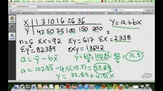
In this video we discuss how to construct draw find a regression line equation, and cover what is a regression line equation. We go through an example of how to calculate a regression line equation by hand. Transcript/notes Once you have determined that the correlation between 2 variables is significant, next is to find the line that best models the data. This line is called a regression line or the line of best fit. And this line is then often times used to predict a value of y, the dependent variable, given a value of x, the independent variable. And the x and y variables are often referred to as the explanatory and response variables. For instance, here is the data set that I have been using in several correlation videos, passing yards in column 1 and points scored in column 2. Here is the scatter plot for that data set, and here is the regression line for the data. And the equation for this regression line is yhat equals 0.0753 times x plus 11.313, which takes on the form of y =’s mx plus b, and we use y hat to show this is a predicted value for y. So,the question is, how was the equation for this line constructed? We can take a closer look at the line and the data points used to determine the line. For instance this point here, has an x value of 313, and a value of 30 for y, which is called the observed value. For that same x value of 313, the yhat value of the line, called the predicted value is 34.89. The differences between the observed values and the predicted values are called residuals, and residuals can be positive, negative or zero. The residuals are often noted with a small d and a subscript. I have added in a third column into the table marking the values of the residuals for each of the 16 ordered pairs. And now I am going to add in a fourth column for the values of the residuals squared and sum it up at the bottom of the column. This total at the bottom is the sum of d squared, which is called the sum of squares of the residuals. And this regression line that is drawn in the scatter plot, is drawn through a set of points where the sum of squares of all the residuals is at a minimum. So, for instance, we could drawn in say 4 other lines, but, for any of these other lines, if we were to square up and sum all of the residuals for each of the lines, they would all be greater than the sum of the squares of the residuals for this line, yhat equals 0.0753 times x plus 11.313. So, this is the line of best fit. Next, we need to look at how do we come up with the actual equation for the line of best fit? At some point in your life you have probably seen this equation; y equals mx plus b, which is the equation of a line. In this equation, m is the slope of the line, and b is the y-intercept of the line. The slope is a ratio, rise over run, so a slope of 3 means that from a point on a line, we rise up 3 units and run over 1 unit, and of course slope can be negative, a slope of negative 3 over 2 means down 3 and over 2. The y-intercept of a line is the point the line crosses the y axis. So, in our passing yards and points example the equation of the line is yhat equals 0.0753 times x plus 11.313. So, the slope is 0.0753 and the y intercept is 11.313. The formula for m, the slope is m equals, n times the sum of x times y, minus the sum of x times the sum of y, divided by, n times the sum of x squared minus the sum of x quantity squared. And in this formula, n is the number of ordered pairs. In our table, we can add in 2 columns, which I have done here, x times y, and x squared. Now we can sum these up at the bottom of the table, and we have everything we need. Plugging into the formula, we get m equals 0.0753, and that is our slope. And the formula for b, the y-intercept is y bar minus m times xbar, or the sum of y over n minus m times the sum of x over n. Plugging into this formula we get 11.313, and that is our y-intercept. Now we can actually use the line to predict. For instance, when a quarterback throws for 325 yards in a game, the predicted points scored is 35.8. Timestamps 0:00 What Is The Line Of Best Fit? 0:22 Regression Line Example Drawn 0:58 Observed And Predicted Values 1:12 What Are Residuals? 1:30 What Is The Sum Of Squares? 2:14 The Slope And Y Intercept 2:49 Formula For The Slope Of A Line 3:19 Formula For The Y Intercept Of A Line 3:38 Using A Regression Line To Predict Values